
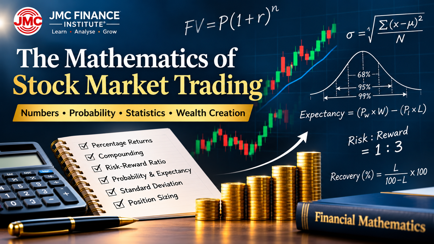
The Mathematics of Stock Market Trading
NUMBERS • PROBABILITY • STATISTICS • WEALTH CREATION
Introduction
The stock market is often viewed as a place where investors make money by identifying the right stocks and traders earn profits by predicting price movements. However, beneath every successful trading decision lies an important foundation: Mathematics.
Stock market trading involves numbers, percentages, probability, statistical analysis, ratios and mathematical relationships. Understanding these concepts can help traders make more disciplined decisions, manage risk and evaluate the effectiveness of their trading strategies.
At JMC Finance Institute, we believe that understanding the mathematics behind financial markets is an important step towards becoming a knowledgeable and disciplined market participant.
1. The Mathematics of Percentage Returns
Every investment decision ultimately involves calculating returns.
Suppose an investor purchases a share at ₹1,000 and sells it at ₹1,100.
Return = (1,100 − 1,000) ÷ 1,000 × 100 = 10%.
2. Why Recovering Losses Requires Higher Returns
One of the most interesting mathematical facts in investing is that the percentage gain required to recover a loss is always greater than the percentage loss.
| Initial Loss | Recovery Required |
|---|---|
| 10% | 11.11% |
| 20% | 25% |
| 30% | 42.86% |
| 40% | 66.67% |
| 50% | 100% |
| 60% | 150% |
| 70% | 233.33% |
Suppose an investor has ₹1,00,000. After a 50% loss, the capital becomes ₹50,000. To return to ₹1,00,000, the investor needs a 100% return on the remaining capital.
3. The Mathematics of Compounding
Compounding is one of the most powerful mathematical principles in wealth creation. It occurs when returns earned on an investment are reinvested, allowing future returns to be earned on a progressively larger capital base.
P = Initial investment
r = Rate of return per period
n = Number of periods
Consider an investment of ₹1,00,000 earning an assumed annual return of 12%.
After five years:
Future Value = 1,00,000 × (1.12)5 = approximately ₹1,76,234.
| Year | Investment Value |
|---|---|
| 0 | ₹1,00,000 |
| 1 | ₹1,12,000 |
| 2 | ₹1,25,440 |
| 3 | ₹1,40,493 |
| 4 | ₹1,57,352 |
| 5 | ₹1,76,234 |
This example assumes a constant annual return, without taxes, fees or withdrawals. Actual market returns fluctuate and are not guaranteed.
4. Understanding Risk-Reward Ratio Mathematically
Suppose a trader purchases a stock at ₹500, keeps a stop loss at ₹480 and sets a target of ₹560.
Risk = ₹500 − ₹480 = ₹20.
Reward = ₹560 − ₹500 = ₹60.
This means the potential reward is three times the amount being risked. However, the probability of winning also matters.
5. The Mathematics of Probability and Trading Success
Consider a trading strategy with the following characteristics:
- Winning trades: 40%
- Losing trades: 60%
- Average profit per winning trade: ₹3,000
- Average loss per losing trade: ₹1,000
For every 100 trades:
Total profit = 40 × ₹3,000 = ₹1,20,000.
Total loss = 60 × ₹1,000 = ₹60,000.
Net profit = ₹60,000.
= (0.40 × 3,000) − (0.60 × 1,000)
= ₹600 per trade.
This demonstrates that a trader does not necessarily need to win most of the trades to have a profitable strategy. The example excludes brokerage, taxes and slippage.
6. Standard Deviation and Stock Market Volatility
Standard deviation is a statistical measure used to understand the dispersion of values around their average. In financial markets, it is commonly used to measure the variability of historical returns.
σ = √[Σ(x − μ)² ÷ N]
σ = Standard deviation
x = Individual observation
μ = Mean of observations
N = Number of observations
A higher standard deviation indicates greater dispersion in returns, while a lower standard deviation indicates relatively lower dispersion.
Historical volatility does not guarantee future volatility, and financial returns do not always follow a normal distribution.
7. The Mathematics of Position Sizing
Suppose a trader has ₹5,00,000 and decides to risk only 1% of capital on a particular trade.
Maximum planned risk = ₹5,00,000 × 1% = ₹5,000.
Entry price = ₹1,000. Stop-loss price = ₹950.
Risk per share = ₹50.
= ₹5,000 ÷ ₹50
= 100 shares
Actual losses can exceed the planned amount because of slippage, market gaps and execution risks.
8. Mathematics Is a Tool, Not a Guarantee
Mathematics can help traders analyse markets objectively, but no mathematical formula can guarantee a successful trade.
Market behaviour is influenced by economic conditions, interest rates, corporate earnings, liquidity, investor psychology, institutional participation and unexpected events.
A mathematical model is only as useful as its assumptions, data and practical application. Mathematical analysis should always be combined with sound risk management and proper evaluation of trading systems.
Conclusion
The stock market is not simply a place where prices move up and down. It is also an environment in which mathematical principles play a significant role.
Percentage calculations, compounding, probability, standard deviation, risk-reward ratios and position sizing are essential concepts for understanding trading and investing.
A disciplined trader should understand not only how much profit can be earned but also how much can be lost, how frequently a strategy succeeds and how capital behaves over time.
Mathematics does not eliminate market risk, but it can help us understand, measure and manage it more intelligently.
Empowering Financial Knowledge Through Research, Mathematics and Technical Analysis.